Tutorial

Example with a 2D Uniform Distribution

This example generates a 2D random uniform distribution. We will use these points to show how you can use Grid and GriSPy to index and query for neighbors.

Keep in mind that the class Grid provides the funcitonality needed to index the points. The class GriSPy inherits from Grid all its functionalities and adds the relevant methods to perform neighbors queries: set_periodicity, bubble_neighbors, shell_neighbors and nearest_neighbors. For completeness, we will show the example using GriSPy.

### Table of Contents

* Create a random distribution of points

* Index the points with Grid/GriSPy

* Creating your curstom distance function

Create a random distribution of points

Import GriSPy and others packages

import numpy as np
import matplotlib.pyplot as plt

import grispy as gsp

Create random points and centres

Npoints = 10 ** 3
Ncentres = 2
dim = 2
Lbox = 100.0

rng = np.random.default_rng(seed=0)
data = rng.uniform(0, Lbox, size=(Npoints, dim))
centres = rng.uniform(0, Lbox, size=(Ncentres, dim))

Index the points with Grid/GriSPy

grid = gsp.GriSPy(data, N_cells=32)

You can get some information about the grid using some helpfull methods:

grid.shape   # number of cells per dimension

(32, 32)

grid.edges   # grid edges in each dimension

array([[2.97613690e-01, 1.90001607e-02],
       [9.99501352e+01, 9.98067457e+01]])

digits = grid.cell_digits(centres)   # check the cell indices (or digits) where a given set of points would fall
digits

array([[31,  1],
       [29,  8]], dtype=int16)

This means that from the 2 input points, the first would be located in the cell (31, 1) and the second in (29, 8).

grid.cell_count(digits)   # number of points in the array `data` that where indexed at initialization

array([2, 0])

grid.cell_centre(digits)    # position of each cell centre

array([[98.39306458,  4.69655073],
       [92.16478198, 26.52512006]])

The digits of cells can be used in other useful methods like cell_walls or cell_points.

Another important method is contains which shows if a given set of new points are contained by the grid.

points = np.array([
    [30., 50.],
    [-10., -10.]
])
grid.contains(points)

array([ True, False])

Set periodicity conditions

Set periodicity conditions on x-axis (or axis=0) and y-axis (or axis=1)

periodic = {0: (0, Lbox), 1: (0, Lbox)}
grid.set_periodicity(periodic, inplace=True)
grid

GriSPy(N_cells=32, copy_data=False, periodic={0: (0, 100.0), 1: (0, 100.0)}, metric='euclid')

Also you can build a periodic grid in the same step

grid = gsp.GriSPy(data, periodic=periodic)

Important: Periodic boundaries don’t have to be exactly the same as the values of grid.edges. The edges of the grid are computed from real data to optimize the queries on sparse data. So, there is nothing wrong on the edge of the grid being at 99.9 but the periodic boundary set exactly at 100.

Query for neighbors within upper_radii

upper_radii = 10.0
bubble_dist, bubble_ind = grid.bubble_neighbors(
    centres, distance_upper_bound=upper_radii
)

Query for neighbors in a shell within lower_radii and upper_radii

upper_radii = 20.0
lower_radii = 10.0
shell_dist, shell_ind = grid.shell_neighbors(
    centres,
    distance_lower_bound=lower_radii,
    distance_upper_bound=upper_radii
)

Query for nth nearest neighbors

n_nearest = 10
near_dist, near_ind = grid.nearest_neighbors(centres, n=n_nearest)

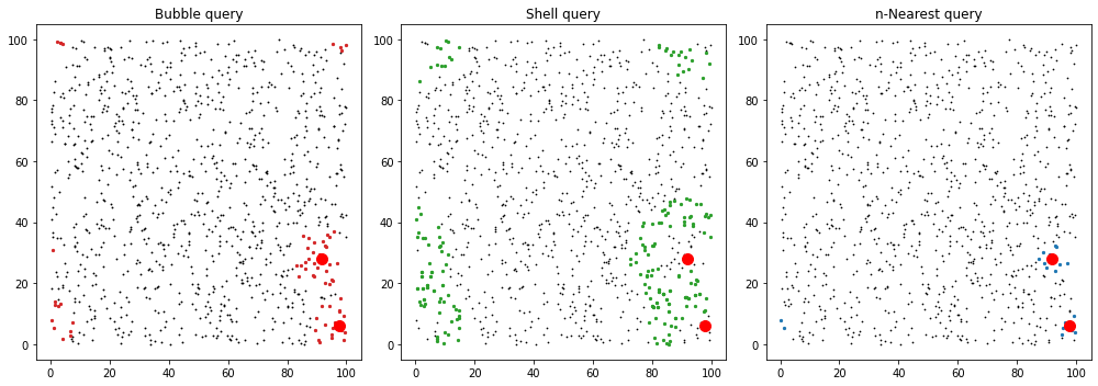
Plot results

fig, axes = plt.subplots(1, 3, figsize=(14, 5))

ax = axes[0]
ax.set_title("Bubble query")
ax.scatter(data[:, 0], data[:, 1], c="k", marker=".", s=3)
for ind in bubble_ind:
    ax.scatter(data[ind, 0], data[ind, 1], c="C3", marker="o", s=5)
ax.plot(centres[:,0],centres[:,1],'ro',ms=10)


ax = axes[1]
ax.set_title("Shell query")
ax.scatter(data[:, 0], data[:, 1], c="k", marker=".", s=2)
for ind in shell_ind:
    ax.scatter(data[ind, 0], data[ind, 1], c="C2", marker="o", s=5)
ax.plot(centres[:,0],centres[:,1],'ro',ms=10)

ax = axes[2]
ax.set_title("n-Nearest query")
ax.scatter(data[:, 0], data[:, 1], c="k", marker=".", s=2)
for ind in near_ind:
    ax.scatter(data[ind, 0], data[ind, 1], c="C0", marker="o", s=5)
ax.plot(centres[:,0],centres[:,1],'ro',ms=10)

fig.tight_layout()

Creating your curstom distance function

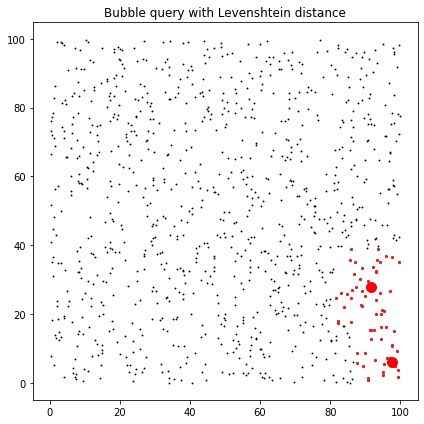
Let’s assume that we intend to compare our distances using levenshtein’s metric for similarity between text (https://en.wikipedia.org/wiki/Levenshtein_distance).

Luckly we have the excellent textdistance library that implements efficiently this distance.

We can install it with

$ pip install textdistance

and then import it with

import textdistance

So to make these custom distance compatible with GriSPy, we must define a function that receives 3 parameters:      - c0 the center to which we seek the distance. - centres the \(C\) centers to which we want to calculate the distance from    a c0. - dim the dimension of each center and c0.

Finally the function must return a np.ndarray with \(C\) elements where the element \(j-nth\) corresponds to the distance between c0 and centres\(_j\).

def levenshtein(c0, centres, dim):
    # textdistance only operates over list and tuples
    c0 = tuple(c0)

    # creates a empty array with the required
    # number of distances
    distances = np.empty(len(centres))
    for idx, c1 in enumerate(centres):

        # textdistance only operates over list and tuples
        c1 = tuple(c1)

        # calculate the distance
        dis = textdistance.levenshtein(c0, c1)

        # store the distance
        distances[idx] = dis

    return distances

Then we create the grid with the custom distance, and run the code

grid = gsp.GriSPy(data, metric=levenshtein)

upper_radii = 10.0
lev_dist, lev_ind = grid.bubble_neighbors(
    centres, distance_upper_bound=upper_radii)

Finally we can check our bubble_neighbors result with a plot

fig, axes = plt.subplots(figsize=(6, 6))

ax = axes
ax.set_title("Bubble query with Levenshtein distance")
ax.scatter(data[:, 0], data[:, 1], c="k", marker=".", s=3)
for ind in lev_ind:
    ax.scatter(data[ind, 0], data[ind, 1], c="C3", marker="o", s=5)
ax.plot(centres[:,0],centres[:,1],'ro',ms=10)

fig.tight_layout()