Tutorial

Example in 2D Uniform Distribution

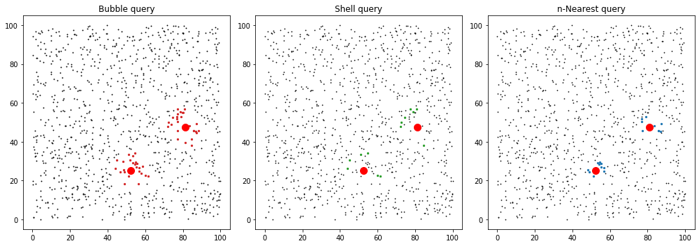
This example generates a 2D random uniform distribution, and then uses GriSPy to search neighbors within a given radius and/or the n-nearest neighbors

---

Import GriSPy and others packages

import numpy as np
import matplotlib.pyplot as plt

from grispy import GriSPy

%matplotlib inline

Create random points and centres

Npoints = 10 ** 3
Ncentres = 2
dim = 2
Lbox = 100.0

np.random.seed(0)
data = np.random.uniform(0, Lbox, size=(Npoints, dim))
centres = np.random.uniform(0, Lbox, size=(Ncentres, dim))

Build the grid with the data

gsp = GriSPy(data)

Set periodicity. Periodic conditions on x-axis (or axis=0) and y-axis (or axis=1)

periodic = {0: (0, Lbox), 1: (0, Lbox)}
gsp.set_periodicity(periodic)

GriSPy(N_cells=20, periodic={0: (0, 100.0), 1: (0, 100.0)}, metric='euclid', copy_data=False)

Also you can build a periodic grid in the same step

gsp = GriSPy(data, periodic=periodic)

Query for neighbors within upper_radii

upper_radii = 10.0
bubble_dist, bubble_ind = gsp.bubble_neighbors(
    centres, distance_upper_bound=upper_radii
)

Query for neighbors in a shell within lower_radii and upper_radii

upper_radii = 10.0
lower_radii = 8.0
shell_dist, shell_ind = gsp.shell_neighbors(
    centres,
    distance_lower_bound=lower_radii,
    distance_upper_bound=upper_radii
)

Query for nth nearest neighbors

n_nearest = 10
near_dist, near_ind = gsp.nearest_neighbors(centres, n=n_nearest)

Plot results

fig, axes = plt.subplots(1, 3, figsize=(14, 5))

ax = axes[0]
ax.set_title("Bubble query")
ax.scatter(data[:, 0], data[:, 1], c="k", marker=".", s=3)
for ind in bubble_ind:
    ax.scatter(data[ind, 0], data[ind, 1], c="C3", marker="o", s=5)
ax.plot(centres[:,0],centres[:,1],'ro',ms=10)


ax = axes[1]
ax.set_title("Shell query")
ax.scatter(data[:, 0], data[:, 1], c="k", marker=".", s=2)
for ind in shell_ind:
    ax.scatter(data[ind, 0], data[ind, 1], c="C2", marker="o", s=5)
ax.plot(centres[:,0],centres[:,1],'ro',ms=10)

ax = axes[2]
ax.set_title("n-Nearest query")
ax.scatter(data[:, 0], data[:, 1], c="k", marker=".", s=2)
for ind in near_ind:
    ax.scatter(data[ind, 0], data[ind, 1], c="C0", marker="o", s=5)
ax.plot(centres[:,0],centres[:,1],'ro',ms=10)

fig.tight_layout()

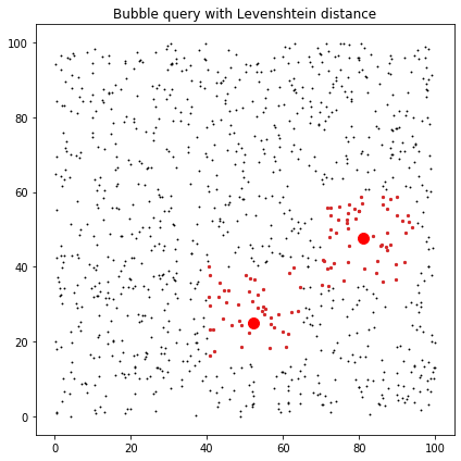
Creating your curstom distance function

Let’s assume that we intend to compare our distances using levenshtein’s metric for similarity between text (https://en.wikipedia.org/wiki/Levenshtein_distance).

Luckly we have the excellent textdistance library that implements efficiently this distance.

We can install it with

$ pip install textdistance

and then import it with

import textdistance

So to make these custom distance compatible with GriSPy, we must define a function that receives 3 parameters:      - c0 the center to which we seek the distance. - centres the \(C\) centers to which we want to calculate the distance from    a c0. - dim the dimension of each center and c0.

Finally the function must return a np.ndarray with \(C\) elements where the element \(j-nth\) corresponds to the distance between c0 and centres\(_j\).

def levenshtein(c0, centres, dim):
    # textdistance only operates over list and tuples
    c0 = tuple(c0)

    # creates a empty array with the required
    # number of distances
    distances = np.empty(len(centres))
    for idx, c1 in enumerate(centres):

        # textdistance only operates over list and tuples
        c1 = tuple(c1)

        # calculate the distance
        dis = textdistance.levenshtein(c0, c1)

        # store the distance
        distances[idx] = dis

    return distances

Then we create the grid with the custom distance, and run the code

gsp = GriSPy(data, metric=levenshtein)

upper_radii = 10.0
lev_dist, lev_ind = gsp.bubble_neighbors(
    centres, distance_upper_bound=upper_radii)

Finally we can check our bubble_neighbors result with a plot

fig, axes = plt.subplots(figsize=(6, 6))

ax = axes
ax.set_title("Bubble query with Levenshtein distance")
ax.scatter(data[:, 0], data[:, 1], c="k", marker=".", s=3)
for ind in lev_ind:
    ax.scatter(data[ind, 0], data[ind, 1], c="C3", marker="o", s=5)
ax.plot(centres[:,0],centres[:,1],'ro',ms=10)

fig.tight_layout()